

So that is done and we can get on with things. In previous episodes we solved a gedanken ionosphere, which was just a homogeneous slab of collisional plasma. How can we extend this result to a solution for the vertically inhomogeneous ionosphere?
Suppose we stack-up a bunch of thin homogeneous slabs of plasma like the one from our gedankenexperiment. If the slabs are sufficiently thin this is a good approximation for the vertically inhomogeneous ionosphere. In Episode II we described a two-mode approximation for the general driven steady-state solution in a single slab, which is parameterized by four complex numbers: the amplitudes of the two modes in each of the two directions, which we might call the “incident” and “reflected” components associated with a source in the magnetosphere. So if we have four boundary conditions that relate the fields in adjacent slabs, and if we know the four amplitudes in one of the slabs, we can calculate the amplitudes in the other slab. Can we somehow use this capability to calculate the input admittance seen from above the ionosphere?
This is actually a standard calculation in transmission line theory. Referring to Episode I, the equivalent circuit for the stack of slabs is the cascade of transmission lines shown in Figure 1. For the one mode case this network can be solved using the transmission line formula that we used in Episode I, except that there I only wrote down the special, open-circuited case when YL = 0. The complete equation 3.88 from Collin (1966) is,

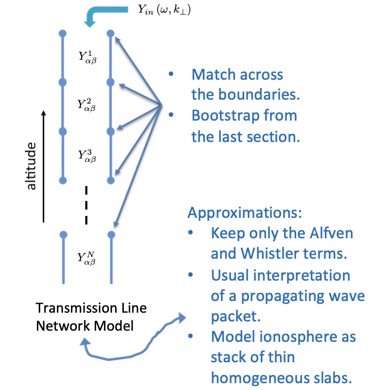
Figure 1: Equivalent circuit for the stack of homogeneous slabs, a cascade of transmission lines. Although normally the characteristic admittances are complex scalars, in our two-mode case we write them as tensors, Yαβ, which are the tensor products of the two polarization vectors of the positive- going modes.
Anyway, what matters at the moment is that equation (1) provides Yin as a function of YL, and so it allows for a recursive solution for the stack of slabs. Since we know that YL = 0 for the last section, we can use equation (1) to find Yin for that section. And since Yin for the last section is YL for the second to last section, we can then apply equation (1) again to obtain Yin for the second-to-last section. And we can repeat this over and over until we get to the top of the stack, which we might call a recursive or bootstrapping solution for the stack of slabs.
The recursive procedure may be generalized for the case of two wave-modes, where now I have to mention that we will use the convention kx = 0, and so the admittance is essentially Bx/Ey, and we can intuit Bx as the parallel current by considering j⃗ ≅∇⃗ × B⃗/μ0. Generally, attaching a lumped-element admittance, Y = Bx/Ey, enforces a ratio of Bx to Ey, and this is equivalent to attaching a semi-infinite piece of transmission line supporting a single propagating mode with polarization vector P = [ Bx, Ey ]. Since the line is infinitely long there is no opportunity for back-reflection, and so Yin is just the characteristic admittance of the wave that is propagating away, Yin = Y0 = Bx/Ey = Y. And this result can also be obtained from equation (1) since as l → ∞, tan kzl → 1/i (assuming ldz is finite).
So maybe we can see that the natural generalization is attachment of a semi-infinite piece of transmission line supporting two wave-modes with polarization vectors P1 = [ B1x, E1y, B1z, E1x ] and P2 = [ B2x, E2y, B2z, E2x ]. We had been assuming (without mention) that Bx and Ey are continuous across the boundaries, but now that we have two modes we will also need to assume that Bz and Ex are continuous, which is the reason we now show them in the polarization vectors. And so, in analogy to finding the “input admittance” for a piece of transmission line attached on top of the first, we should find the equivalent polarization vectors for the equivalent wave-modes that propagate in an equivalent semi-infinite piece of transmission line, which replaces the two pieces.
The four boundary conditions (continuity of Bx, Ey, Bz, and Ex) provide four linear equations that relate the six amplitudes that are at-play on the boundary between any of the two pieces of line in our recursive procedure: the two transmitted amplitudes, the two reflected amplitudes, and the two incident amplitudes. So if we choose the incident amplitudes we can compute the others. For example, we could choose the amplitude for one of the incident modes to be 1 + i0 while choosing the other to be 0 + i0, and then compute the reflected components in both modes. Since these same reflected components are always going to accompany that incident mode, we might as well just pretend that the reflected components are part of the incident mode and that there is no reflection. That is, we can just add up all these components at the input to the two line-sections and pretend that the resultant is the polarization vector for an effective mode in an effective semi-infinite transmission line, which replaces the two pieces. After doing this for both modes, we can move to the next section and do it again, until we reach the top of the stack.
After reaching the top of the stack the entire, vertically-inhomogeneous ionosphere is represented by an equivalent semi-infinite piece of transmission line. We can calculate the reflected components for a particular incident signal, and thus determine all the amplitudes in the region above the ionosphere. And then we can apply the boundary conditions again in reverse-order to transfer these amplitudes back down through the slabs, and resolve the fields inside the ionosphere. In the results presented below we assume the incident signal is an (shear-mode) Alfven wave (for the reasons explained in Episode II), and so the bi-modal nature of the interaction is confined within the ionosphere, and we obtain a single unique quantity for the ionospheric conductance.
Depending on your tolerance for nebulosity, there may be too many omitted details for you to feel really comfortable with this explanation. And although it is rigorously required that Ey, Bz, and Ex are continuous, there may be some of you who are curious about assuming that Bx is continuous, which really amounts to assuming that parallel current is continuous. But the details are in Section 5 of Cosgrove (2022), aka the Supplementary Information for Cosgrove (2024), and so I’m going to proclaim victory: we have solved the system of stacked slabs!

Figure 2: Validation showing agreement between the downward looking conductance and the downward field- line-integral of conductivity (top), and showing perfect mapping of the electric field (bottom, blue), along with the gradual falloff of the magnetic field (bottom, red), which is essentially the parallel current.
I have implemented all of this in some Python/Numpy code, and in order to ensure that everything is as expected, the first step is a validation where I artificially modify the two wave-modes so that both of them satisfy the electrostatic criteria from Episode I. I lengthen the parallel wavelengths and dissipation scale lengths, and I rescale the Eys (in the polarization vectors) so that the wave-Pedersen conductivities equal the usual Pedersen conductivity. As long as the parallel wavelength and dissipation scale length are the same for the two modes, the results are as shown in Figure 2, where the top panel compares the downward looking input admittance to the downward field-line-integral of conductivity, and the bottom panel shows Ey and parallel current (actually Bx), all plotted versus altitude. As expected, the real part of the input admittance matches the field line integrated conductivity, the imaginary part is zero, and the electric field maps perfectly through the ionosphere. So everything seems to be in order and we can proceed to the real waves.
When the real waves are used the results come out quite differently. Figure 3 shows the same two plots for four different cases, using two different electron densities and two different transverse wavelengths (4.7 × 10⁹ m-3 [left], 1.0 × 10¹¹ m-3 [right], 100 km [top], 1000 km [bottom]). Note that the densities are kept constant with altitude, which choice was made to simplify interpretation of the results.
 |
| Figure 3: Results for four different cases using the real waves; with constant densities of 4.7 × 10⁹ m-3 (left), and 1.0 × 10¹¹ m-3 (right); and with transverse wavelengths of 100 km (top), and 1000 km (bottom). The same quantities are plotted as in Figure 2. Note, the frequency in this and all the examples herein is determined from the transverse wavelength and assuming a 40 m/s transverse phase velocity. The resulting periods range from 41.7 minutes to 417 minutes. |
With respect to the comparison of ionospheric conductance to field-line-integrated conductivity, the low-density short-wavelength case agrees pretty well. Surprisingly well, actually, considering that in Episode II we found that the wave-Pedersen conductivity is only about half of the usual Pedersen conductivity. But the explanation is found in the plot of electric field, which rather than mapping unchanged, has a rather large peak near the bottom. This peak may be compensating for the lower conductivity, and so the agreement for conductance appears to be something of a coincidence that arises for this particular case, which was in fact selected for that reason.
Looking to the higher-density, short-wavelength case on the right, increasing the density shortens the parallel wavelength and introduces a resonance effect, where the conductance actually changes sign. While bizarre, this is more like what we expected. The possibility of such a resonance was noted in the conclusion of Episode I, and predicted by the phase rotation results in Episode II. And the shape looks quite a bit like the tangent function in equation (1) of Episode I.
What was not anticipated is the effects at the longer transverse wavelength, where although there is no resonance, there is instead a large reduction in the ionospheric conductance, as compared with the field-line-integrated conductivity. We had been expecting a reduction of about 50%, due to the conductivity difference found in Episode II. But the reduction is closer to 70% or 80%.
To better understand these results we look at the plots of electric field. Especially for the longer transverse wavelength, the electric field cuts-off sharply well above the bottom of the conducting ionosphere. And although there is a slight peak right before the cutoff, this peak isn’t nearly as big in the longer wavelength cases. So in these cases there may be an additional reduction in conductance due to a lack of penetration of the signal; the conductivity at lower altitudes is not contributing to the total ionospheric conductance, as it had hitherto been expected to do.

The cutoff appears to be the result of a strong modal interaction that may be diagnosed by looking at
Figure 4, where I have stacked up a bunch of altitude-resolved plots for the 1000 km wavelength case with density 4.7 × 10⁹ m-3. Shown from top to bottom are (1) the input admittance; (2) Ey and Bx; (3) the parallel wavelength for both modes; (4) the characteristic admittance for both modes; and (5) the complex-conjugate dot-product of the two polarization vectors (including all 16 components). What is apparent is that all of the panels show kinky features, and (excepting one) they all line up with a very sharp peak in the alignment of the two modes (bottom panel). It appears that the two modes are degenerating over a very narrow range of altitude, and becoming nearly identical at one specific altitude. (Note, the kink in Panel d actually arises from a different cause, and this panel is shown to support the finding of degeneracy.) The nearly identical modes interact strongly and create a sharp reflection of the signal, so that it does not get passed the altitude of the (near?) degeneracy.
So that completes the major results. Except, before closing out Episode III there is one more plot I am bound to show, which is about if we really need to use the fully electromagnetic waves. At least at smaller scales, it is common to use what are sometimes called electrostatic waves, meaning that the Poisson equation is substituted for the Maxwell equations. This is just a modification of the matrix H5 from Episode II, so we can use exactly the same methods. Figure 5 shows parallel wavelength including the four electromagnetic wave-modes identified in Episode II, together with all the electrostatic modes capable of propagating (wave-modes) for the scale-sizes and frequencies that we consider (see Figure 3 caption). The first finding is that there is one fewer electrostatic wave-mode, and so we need to find out which mode is missing. It is seen that the wavelengths of the electrostatic analogues agree very well for the Ion and Thermal modes. And for transverse wavelengths less than about 100 m there is also good agreement for the Alfven mode. So the missing mode appears to be the Whistler wave. And as to the analogue for the Alfven wave, above about 100 m its parallel wavelength is orders of magnitude too long.

top panel shows parallel wavelength versus altitude for a 100 km transverse wavelength, and the bottom panel shows parallel wavelength versus perpendicular wavelength for a 145 km altitude (ne = 1011 m-3). There is no trace for the electrostatic analogue to the Whistler wave, because no other propagating modes could be found for this range of transverse wavelength and frequency (see caption to Figure 3 for frequency information).
Since the Whistler wave does not propagate at the shorter transverse wavelengths (bottom panel of Figure 5), it remains possible that the electrostatic waves provide good substitutes for transverse wavelengths less than about 100 m, which is where they are most-commonly used. But for the kilometer-scale transverse wavelengths that we have been investigating, using the electrostatic analogues will give very different results. The short wavelength effects such as the resonance will be missing. And the modal interaction that cuts-off the electric field will also be missing.
And so that’s pretty much that, and I’m not sure if it seems abrupt or like its been going on forever. One thing I’ve been realizing, I probably should not have chosen the word “debunking” for the title of these blogs because it sounds sort of iconoclastic, and one of the referees criticized me for this. I regret that choice. Electrostatic theory is an important baseline that gives us something to compare with
the new baseline, that we have developed here. And it is included in electromagnetic theory as a special case. Since this point seems to be beyond me, here is what Albert Einstein had to say about the fate of electrostatic theory, which he hoped would also follow for the special theory of relativity (Einstein, 1916). It is translated from the German but it still sounds good,
It is just that the ionosphere does not appear to achieve this limit. The electromagnetic fluid equations appear to override the major predictions of electrostatic theory. The ionospheric conductance is not the field line integrated conductivity. The parallel wavelength is not long enough to be ignored. The electric field does not map through ionosphere. There are instead electromagnetic waves that enter the ionosphere, couple into other electromagnetic modes, rattle around, and eventually come to a steady-state involving a lot more richness than was previously expected for ionospheric phenomena.
For lovers of the ionosphere, those who have on certain occasions braved the polar bears to switch-on the ISR, or waited all night for that perfect moment to launch the rockets, or dreamed of a satellite that could go lower, or of a lidar that could see higher, or who spread out the cameras as far as they could, or the magnetometers, or the ionosondes, or the CSRs, or the GPSs, or the FPIs, or even the riometers, this is wonderful! Long live the ionosphere!!

by Russell Bonner Cosgrove
References
Collin, R. E. (1966), Foundations for Microwave Engineering, McGraw-Hill.
Cosgrove, R. B. (2022), An electromagnetic calculation of ionospheric conductance that seems to override thefield line integrated conductivity, Zenodo and ArXiv, doi: https://doi.org/10.48550/ARXIV.2211.10818, https://doi.org/10.5281/Zenodo.7416494.Cosgrove, R. B. (2024), On an electromagnetic calculation of ionospheric conductance that seems to override the field line integrated conductivity, Sci Rep, 14(7701), doi: https://doi.org/10.1038/s41598-024-58512-x.
Einstein, A. (1916), Relativity the special and general theory, 15 ed., Crown Publishers, INC.


