• Photo by Nicolas J Leclercq on Unsplash
  • Photo by Nicolas Tissot on Unsplash
  • Photo by NASA on Unsplash
  • Photo by USGS on Unsplash
Showing posts with label series3. Show all posts

A new view of lunar magnetism

One of the enduring mysteries about the Moon is whether it ever had an internal-generated magnetic field, and if so, when the core dynamo ceased. New research by Tinghong Zhou, John Tarduno, Rory Cottrell, and Eric Blackman at the University of Rochester and collaborators from the University of Notre Dame, UC Santa Cruz, and the University of Arizona, in a study supported by NSF and NASA, have provided new insights into this lunar puzzle, narrowing down the potential lifespan of the Moon’s dynamo to its first ~140 million years. The new study focused on analyzing magnetic field intensity (called paleointensity) recorded in Apollo samples that are between 4.36 to 3.7 billion years old. Using an advanced technique known as single-crystal paleointensity analysis, the researchers were able to obtain accurate measurements of the Moon’s ancient ambient surface magnetic field environment – which indicated negligible field strengths. This evidence for the absence of a dynamo resolves the long-lasting paradox between the previously hypothesized long-lived lunar dynamo and energy considerations, namely that the tiny lunar core would have been unable to power a strong, sustained magnetic field.

Figure 1: Astronaut John Young stands on the rim of the Plum Crater on the Moon. Image source: NASA, Apollo Lunar Surface Journal, Apollo Image Library Hasselblad Magazine, 109/G (B&W), AS16-109-17804.

A key part of this new understanding of lunar magnetic history comes from a focus on magnetic carriers meeting the demanding requirements of paleointensity theory. Single-domain magnetic grains, which are very small, some 20 to 200 nm in size, are required. In contrast, larger magnetic grains are far less reliable because their internal domain walls can move with time and during laboratory treatments, corrupting any original magnetic signal. Magnetic minerals in lunar rocks are dominated by these problematic multidomain grains, making paleointensity analysis very challenging. The single-crystal paleointensity technique used in the study by Zhou and others builds on an earlier study led by the University of Rochester and focuses on silicate crystals that contain single-domain magnetic grain inclusions to meet the paleointensity recording requirement. The authors tested the fidelity of their records by CO2 laser heating in different fields and in the presence or absence of an applied field. These tests exclude thermal alteration and provide a measure of recording efficiency. The authors found high recording efficiencies, indicating that if surface fields had been present, they would have been recorded. Hence, the absence of a paleointensity indicates absence of a surface field.

In addition to the single crystal paleointensity, the study also employed whole rock paleointensity on 3.7-billion-year-old Apollo basalts using a non-thermal technique. Unlike thermal methods that measure magnetization acquired from natural cooling, non-thermal methods rely on additional assumptions and empirical calibrations. The results from the non-thermal technique showed abnormally high and inconsistent paleointensities. These anomalies could indicate shock magnetization from lunar impacts or issues with the multidomain grains and/or the applied non-thermal method. Because non-thermal analysis of whole rocks is the basis for some calls for an episodic lunar dynamo, the researchers conclude there is no robust evidence for such a phenomenon from Apollo samples.

Figure 2: Lunar magnetic history indicated by paleointensity data. Single crystals suggest a null lunar magnetic field since 4.36 Ga, while some whole rock data obtained by non-thermal methods yield abnormally high values that might be related to large multidomain magnetic grains and/or impact induced magnetic field. Figure modified from Tarduno et al., 2021 and Zhou et al., 2024.

If the Moon did not have a dynamo for most of its history, the early Earth’s (for example, during the Archean and Hadean eons) atmosphere can be transferred to the Moon, which would be unshielded by an intrinsic field, and preserved in its regolith. With a smaller Earth-Moon distance and the stronger solar wind in the Archean and Hadean, this transfer would have been enhanced. By studying the volatiles trapped in the lunar regolith, we might have opportunities to better understand the composition of the early Earth’s atmosphere and the conditions that influenced the evolution of life.


Tinghong Zhou is a postdoctoral researcher at the University of Rochester mentored by Professor John A. Tarduno. Her research focuses on the long-term evolution of the geomagnetic field and its correlation with the Earth’s deep interior, and the origin of the lunar magnetism. Email address: tzhou16@ur.rochester.edu

Not all who wander are lost – updating the International Geomagnetic Reference Field

The Earth’s magnetic field is not static and varies on many different time scales. The main source of the long-term field variation comes from the outer core where the magnetic field is generated by the motion of liquid nickel-iron which in turn ‘drags’ the field lines with it. Thus, the field changes strength and shape slowly over decades. Every five years, IAGA issues an updated version of the magnetic field to capture these slow changes known as secular variation. This series of ‘maps’ or models are known as the International Geomagnetic Reference Field (IGRF) and goes back 125 years. In November 2024, the 14th generation of the model was released, valid from January 1900 to December 2030.

Figure 1: Strength of the magnetic field in microTelsa on the Earth’s surface at 2025.0. Note the low strength region known as the South Atlantic Anomaly.

The magnetic field is represented by a series of numbers known as Gauss coefficients. Using the mathematical technique of spherical harmonic analysis, the magnetic field can be represented continuously in time and space rather than as a 3D grid of cells. This means we can provide a snapshot of the magnetic field above, at or below the Earth’s surface using a very compact set of just 195 numbers, which gives an approximate resolution of 3000 km. This captures the vast majority of the core field and allows us to calculate of Declination angle, Magnetic Dip and Total Field Intensity (see Figure 1) anywhere in the world. We can also track the location of the magnetic poles (see Figure 2).

The first IGRF for 1965 was issued in 1968 when it was difficult to get timely datasets of magnetic measurements from observatories – the data usually took several years to produce and was distributed by post! When the modern internet era began in the 1990s, data could be circulated more rapidly and the IGRF began to be produced in a more timely fashion. Today, we live in a golden era of magnetic field measurement: from hundreds of high-quality geomagnetic observatories to dedicated magnetic missions such as ESA Swarm and Macau Science Satellite. Together these freely available, near-real-time datasets and cheap powerful computer make core field modelling widely accessible.

Figure 2: Estimated location of the geomagnetic and magnetic dip poles from 1900 to 2030. While the north dip pole has accelerated over the past 20 years moving from Canada toward Siberia, the south dip pole has moved much more slowly.

For the 14th generation, 19 teams of geomagnetic scientists from four continents submitted candidate models for the magnetic field in 2020 and 2025 and a forecast of secular variation between 2025 and 2030. In total, there were 47 candidate models to evaluate. The method for combination was determined by a panel of experts using a variety of different technical analyses. The final models were agreed by majority vote and the new coefficients were issued to the official IAGA website on 20th November 2024.

The IGRF is used for research for deep Earth and space weather forecasting, part of many industry applications for correcting surveys (archaeology, oil/gas, mineral exploration) as well as standard pointing and navigation uses. The IGRF truly is an international effort involving thousands of observers, scientists and engineers from around the world. Without their contributions, this would not be possible. We thank them all for their work.


Authors: Ciaran Beggan is senior researcher at British Geological Survey in Edinburgh. This is his fourth venture with the IGRF, starting as a PhD student back in 2009. Clemens Kloss is a postdoctoral researcher at DTU Space in Copenhagen who specialises in improving our view of the Earth’s core magnetic field minus the annoying effects of the aurora.

Exploration of the Jovian system #2

There are two icy moon missions of this decade that will reach their respective bodies of interest beginning of next decade- JUpiter ICy moons Explorer (JUICE) and Europa Clipper. The main focus of JUICE is Ganymede and for Clipper is Europa. Both these planetary bodies are moons of our Solar System's largest planet Jupiter. Scientists are particularly interested in the Jovian moons because these bodies contain large oceans under their surface making them a suitable place to study for potential habitability. They are called 'icy moons' because their surface is made up of ice! If you are interested to learn more about these moons, head to our previous blogs about them!

While JUICE launched on April 14th 2023, Clipper is all set to launch this month! If you are a space enthusiast and are interested in watching the launch: in person- head to Kennedy Space Center in Florida, USA, or online: head to NASA's website. The launch window starts within a week on October 10th and goes up till the end of the month. It will take Clipper five and a half years to reach Jupiter in 2030.

Image Credit: NASA

STFC Introductory Course

The STFC (Science and Technology Facilities Council) Introductory Course in Solar and Solar-Terrestrial Physics was held at the University of Sheffield, UK from September 2nd to 6th, 2023. This annual course, organised by the UK Solar Physics and MIST (Magnetospheric, Ionospheric, and Solar-Terrestrial) Councils, and approved by the Heads of UK Solar Groups and MIST since 2015, continues to play a crucial role in training early career UK solar system physicists. While most of this year’s participants were from the UK, we were pleased to welcome students from Hungary, Germany, France, India, China, and South Korea, adding a truly international dimension to the event.

This summer school is specifically designed for PhD students who are new to the field, with the aim of helping them upgrade, consolidate, and broaden their knowledge. The program covered a wide range of essential topics in Sun-Earth connections. After each lecture, there was a longer break with coffee and biscuits, providing students an opportunity to engage with the lecturers in a more informal and relaxed environment. Alongside these subject-specific lectures, students also benefited from sessions focusing on career development and public engagement.


A highlight of the course was the careers panel, featuring professionals from diverse backgrounds and at various stages of their careers. The panel included individuals who followed a straight academic path from their Master’s degrees to becoming professors, as well as those who took time away from academia before returning to pursue a PhD and continuing in research. Each panel member shared their unique career journey, offering students different perspectives on navigating both academic and non-academic careers. After sharing their stories, the panel opened the floor for questions, leading to a lively and insightful discussion. Students asked the panelists what they might have done differently, and what advice they would offer to those just starting out. The candid responses provided practical guidance and encouragement, helping students think more clearly about their own career paths and future challenges.

The public engagement talk was equally inspiring, as the speaker shared her extensive experience in conducting outreach activities across the globe. Her insights showed the importance of public engagement and demonstrated how impactful outreach can be for both scientists and the broader community.


- Marianna B. Korsos, Leverhulme Early Career Fellow, University of Sheffield

ESA's Planetary Science Archive (PSA)

Wondering where to find, or even if you can use at all, science data from the European Space Agency’s Solar System missions?

This is where you need to go -->  https://psa.esa.int !

The European Space Agency's past and current Solar System space missions have produced, and continue to produce, tons of data for scientific use, which are available in ESA's Planetary Science Archive (PSA) and can be accessed through the web user interface (web UI) at https://psa.esa.int.

PSA data products are all scientifically peer-reviewed in the Planetary Data System (PDS) standard with the aim of preserving the data for the long term, having in view the use of new techniques or methodologies that are not available when the missions are carried out. Space missions with data in the PSA include BepiColombo, ExoMars Trace Gas Orbiter, Giotto, Huygens, Juice, Mars Express, Rosetta, SMART-1 and Venus Express.

The web UI provides search by mission, target, instrument type, processing level, observational geometry and other parameters, so you can easily find the data you are looking for. This interface also allows a user to skim through "browse" data products, which give a quick, visual, snapshot of the data. In addition, where possible, map-based searches in 2D and 3D are possible. The web UI is supplemented by programmatic interfaces (APIs) and a secure FTP server. All of these services are under constant evolution and your feedback is greatly appreciated on how we can improve.


Joana S. Oliveira is an archive scientist working for the European Space Agency (ESA) JUICE and Heliophysics missions, with a background in planetary sciences. She is interested in learning about the history of rocky planets through their magnetic field signals.


Where is the magnetized material located on the lunar surface?

Magnetometers onboard spacecraft have detected magnetic field signals originating from the lunar crust. These signals are known as magnetic anomalies and are generated by rocks that are permanently magnetized. Lunar magnetic anomalies are distributed heterogeneously over the lunar surface and the geological processes that gave rise to them is under debate. Thus, the Moon's geological history can be further assessed by inferring the shape of the underlying magnetized material. Up to now, these sources were not fully described for such geological assessment studies.

Joana Oliveira and her colleagues, in a recently published work, evaluated the ability of a methodology up to now used to infer the direction of the magnetization, called the method of Parker, to recover the location and shape of the magnetized material by using orbital magnetic field data only.


Lunar magnetic field map at 30 km altitude using Tsunakawa et al. 2015 model.

Through a series of tests, the authors of this study have shown that the Parker’s method can constrain the shape of the source of a magnetic anomaly, provided that the respective part of the crust is magnetized along a common direction.

"We tried to take it a step further to crack the unidirectional assumption by testing complex bodies with different directions, and we were surprised by how this method was still able to recover most of the magnetized structure”, Joana said.

The authors also applied the method to two lunar magnetic anomalies related to two visible geological features an impact crater and an albedo anomaly, also know by swirls. Results show that the inferred shape and location of the magnetized material are in good agreement with the associated geological features and suggest that one originated by an impact event and the other by volcanic activity.


Parker inversion results for the Mendal-Rydberg basin. The magnetized material (related to the dipole moments) is correlated with the inner depression in blue color of the topography map, despite the magnetic field signal being shifted to the southwest from the center of the basin. Figure adapted from Oliveira et al. 2024.

Future applications can focus on constraining the origin of the many lunar magnetic anomalies that are not associated with visible geological features.


Joana S. Oliveira is an archive scientist working for the European Space Agency (ESA) JUICE and Heliophysics missions, with a background in planetary sciences. She is interested in learning about the history of rocky planets through their magnetic field signals.

Debunking a Pillar of Ionospheric Science, and Building a New One: Episode III

Hello dear reader and thank you for attending to these blogs, which was certainly not your easiest option. I am giving myself a second to think about where you might be and what might be your surroundings. We have such a wonderfully global community! I would like to say that “It’s all good.”, which of course is both true and false, depending on what perspective we choose to adopt. There is a very particular perspective intended for these blogs, and it is a rather heady one: we adopt the laws of physics as they are currently understood by humans, and we apply them to the question of electricity in the ionosphere. About that, I think our saga is nearing completion. There is some good news in that, hey!, the Cosgrove (2022) preprint has been published in Scientific Reports!! Well actually the preprint is the Supplementary Information for the much shorter Scientific Reports paper, which is probably just how things ought to be.

So that is done and we can get on with things. In previous episodes we solved a gedanken ionosphere, which was just a homogeneous slab of collisional plasma. How can we extend this result to a solution for the vertically inhomogeneous ionosphere?

Suppose we stack-up a bunch of thin homogeneous slabs of plasma like the one from our gedankenexperiment. If the slabs are sufficiently thin this is a good approximation for the vertically inhomogeneous ionosphere. In Episode II we described a two-mode approximation for the general driven steady-state solution in a single slab, which is parameterized by four complex numbers: the amplitudes of the two modes in each of the two directions, which we might call the “incident” and “reflected” components associated with a source in the magnetosphere. So if we have four boundary conditions that relate the fields in adjacent slabs, and if we know the four amplitudes in one of the slabs, we can calculate the amplitudes in the other slab. Can we somehow use this capability to calculate the input admittance seen from above the ionosphere?

This is actually a standard calculation in transmission line theory. Referring to Episode I, the equivalent circuit for the stack of slabs is the cascade of transmission lines shown in Figure 1. For the one mode case this network can be solved using the transmission line formula that we used in Episode I, except that there I only wrote down the special, open-circuited case when YL = 0. The complete equation 3.88 from Collin (1966) is,

where YL is an arbitrary load admittance,  
kz 2π/λz − i/ldzλis the parallel wavelength, ldz is the dissipation scale length, Y0 is the characteristic admittance of the wave, and l is the length of the line. Isn’t it beautiful! It is amazing the complexity that arises from a single piece of transmission line! This would be a good time to remember the Smith chart from Episode I.

Figure 1: Equivalent circuit for the stack of homogeneous slabs, a cascade of transmission lines. Although normally the characteristic admittances are complex scalars, in our two-mode case we write them as tensors, Yαβ, which are the tensor products of the two polarization vectors of the positive- going modes.

Anyway, what matters at the moment is that equation (1) provides Yin as a function of YL, and so it allows for a recursive solution for the stack of slabs. Since we know that YL = 0 for the last section, we can use equation (1) to find Yin for that section. And since Yin for the last section is YL for the second to last section, we can then apply equation (1) again to obtain Yin for the second-to-last section. And we can repeat this over and over until we get to the top of the stack, which we might call a recursive or bootstrapping solution for the stack of slabs.

The recursive procedure may be generalized for the case of two wave-modes, where now I have to mention that we will use the convention kx = 0, and so the admittance is essentially Bx/Ey, and we can intuit Bx as the parallel current by considering  j⃗ ∇⃗ × B⃗/μ0Generally, attaching a lumped-element admittance, Y = Bx/Ey, enforces a ratio of Bx to Ey, and this is equivalent to attaching a semi-infinite piece of transmission line supporting a single propagating mode with polarization vector P = [ BxEy ]. Since the line is infinitely long there is no opportunity for back-reflection, and so Yin is just the characteristic admittance of the wave that is propagating away, Yin = Y0 = Bx/Ey = Y. And this result can also be obtained from equation (1) since as l → ∞, tan kzl → 1/i (assuming ldz is finite).

So maybe we can see that the natural generalization is attachment of a semi-infinite piece of transmission line supporting two wave-modes with polarization vectors P1 = [ B1xE1y, B1zE1] and P2 = [ B2xE2y, B2zE2]. We had been assuming (without mention) that Bx and Ey are continuous across the boundaries, but now that we have two modes we will also need to assume that Bz and Ex are continuous, which is the reason we now show them in the polarization vectors. And so, in analogy to finding the “input admittance” for a piece of transmission line attached on top of the first, we should find the equivalent polarization vectors for the equivalent wave-modes that propagate in an equivalent semi-infinite piece of transmission line, which replaces the two pieces.

The four boundary conditions (continuity of BxEyBz, and Ex) provide four linear equations that relate the six amplitudes that are at-play on the boundary between any of the two pieces of line in our recursive procedure: the two transmitted amplitudes, the two reflected amplitudes, and the two incident amplitudes. So if we choose the incident amplitudes we can compute the others. For example, we could choose the amplitude for one of the incident modes to be 1 + i0 while choosing the other to be 0 + i0, and then compute the reflected components in both modes. Since these same reflected components are always going to accompany that incident mode, we might as well just pretend that the reflected components are part of the incident mode and that there is no reflection. That is, we can just add up all these components at the input to the two line-sections and pretend that the resultant is the polarization vector for an effective mode in an effective semi-infinite transmission line, which replaces the two pieces. After doing this for both modes, we can move to the next section and do it again, until we reach the top of the stack.

After reaching the top of the stack the entire, vertically-inhomogeneous ionosphere is represented by an equivalent semi-infinite piece of transmission line. We can calculate the reflected components for a particular incident signal, and thus determine all the amplitudes in the region above the ionosphere. And then we can apply the boundary conditions again in reverse-order to transfer these amplitudes back down through the slabs, and resolve the fields inside the ionosphere. In the results presented below we assume the incident signal is an (shear-mode) Alfven wave (for the reasons explained in Episode II), and so the bi-modal nature of the interaction is confined within the ionosphere, and we obtain a single unique quantity for the ionospheric conductance.

Depending on your tolerance for nebulosity, there may be too many omitted details for you to feel really comfortable with this explanation. And although it is rigorously required that EyBz, and Eare continuous, there may be some of you who are curious about assuming that Bx is continuous, which really amounts to assuming that parallel current is continuous. But the details are in Section 5 of Cosgrove (2022), aka the Supplementary Information for Cosgrove (2024), and so I’m going to proclaim victory: we have solved the system of stacked slabs!

Figure 2: Validation showing agreement between the downward looking conductance and the downward field- line-integral of conductivity (top), and showing perfect mapping of the electric field (bottom, blue), along with the gradual falloff of the magnetic field (bottom, red), which is essentially the parallel current.

I have implemented all of this in some Python/Numpy code, and in order to ensure that everything is as expected, the first step is a validation where I artificially modify the two wave-modes so that both of them satisfy the electrostatic criteria from Episode I. I lengthen the parallel wavelengths and dissipation scale lengths, and I rescale the Eys (in the polarization vectors) so that the wave-Pedersen conductivities equal the usual Pedersen conductivity. As long as the parallel wavelength and dissipation scale length are the same for the two modes, the results are as shown in Figure 2, where the top panel compares the downward looking input admittance to the downward field-line-integral of conductivity, and the bottom panel shows Ey and parallel current (actually Bx), all plotted versus altitude. As expected, the real part of the input admittance matches the field line integrated conductivity, the imaginary part is zero, and the electric field maps perfectly through the ionosphere. So everything seems to be in order and we can proceed to the real waves.

When the real waves are used the results come out quite differently. Figure 3 shows the same two plots for four different cases, using two different electron densities and two different transverse wavelengths (4.7 × 10⁹ m-3 [left], 1.0 × 10¹¹ m-3 [right], 100 km [top], 1000 km [bottom]). Note that the densities are kept constant with altitude, which choice was made to simplify interpretation of the results.

Figure 3: Results for four different cases using the real waves; with constant densities of 4.7 × 10⁹ m-3 (left), and 1.0 × 10¹¹ m-3 (right); and with transverse wavelengths of 100 km (top), and 1000 km (bottom). The same quantities are plotted as in Figure 2. Note, the frequency in this and all the examples herein is determined from the transverse wavelength and assuming a 40 m/s transverse phase velocity. The resulting periods range from 41.7 minutes to 417 minutes.

With respect to the comparison of ionospheric conductance to field-line-integrated conductivity, the low-density short-wavelength case agrees pretty well. Surprisingly well, actually, considering that in Episode II we found that the wave-Pedersen conductivity is only about half of the usual Pedersen conductivity. But the explanation is found in the plot of electric field, which rather than mapping unchanged, has a rather large peak near the bottom. This peak may be compensating for the lower conductivity, and so the agreement for conductance appears to be something of a coincidence that arises for this particular case, which was in fact selected for that reason.

Looking to the higher-density, short-wavelength case on the right, increasing the density shortens the parallel wavelength and introduces a resonance effect, where the conductance actually changes sign. While bizarre, this is more like what we expected. The possibility of such a resonance was noted in the conclusion of Episode I, and predicted by the phase rotation results in Episode II. And the shape looks quite a bit like the tangent function in equation (1) of Episode I.

What was not anticipated is the effects at the longer transverse wavelength, where although there is no resonance, there is instead a large reduction in the ionospheric conductance, as compared with the field-line-integrated conductivity. We had been expecting a reduction of about 50%, due to the conductivity difference found in Episode II. But the reduction is closer to 70% or 80%.

To better understand these results we look at the plots of electric field. Especially for the longer transverse wavelength, the electric field cuts-off sharply well above the bottom of the conducting ionosphere. And although there is a slight peak right before the cutoff, this peak isn’t nearly as big in the longer wavelength cases. So in these cases there may be an additional reduction in conductance due to a lack of penetration of the signal; the conductivity at lower altitudes is not contributing to the total ionospheric conductance, as it had hitherto been expected to do.

Figure 4: Explanation for the electric field cutoff, which is found in the (near?) degeneracy of the wave-modes.

The cutoff appears to be the result of a strong modal interaction that may be diagnosed by looking at
Figure 4, where I have stacked up a bunch of altitude-resolved plots for the 1000 km wavelength case with density 4.7 × 10⁹ m-3. Shown from top to bottom are (1) the input admittance; (2) Eand Bx; (3) the parallel wavelength for both modes; (4) the characteristic admittance for both modes; and (5) the complex-conjugate dot-product of the two polarization vectors (including all 16 components). What is apparent is that all of the panels show kinky features, and (excepting one) they all line up with a very sharp peak in the alignment of the two modes (bottom panel). It appears that the two modes are degenerating over a very narrow range of altitude, and becoming nearly identical at one specific altitude. (Note, the kink in Panel d actually arises from a different cause, and this panel is shown to support the finding of degeneracy.) The nearly identical modes interact strongly and create a sharp reflection of the signal, so that it does not get passed the altitude of the (near?) degeneracy.

So that completes the major results. Except, before closing out Episode III there is one more plot I am bound to show, which is about if we really need to use the fully electromagnetic waves. At least at smaller scales, it is common to use what are sometimes called electrostatic waves, meaning that the Poisson equation is substituted for the Maxwell equations. This is just a modification of the matrix H5 from Episode II, so we can use exactly the same methods. Figure 5 shows parallel wavelength including the four electromagnetic wave-modes identified in Episode II, together with all the electrostatic modes capable of propagating (wave-modes) for the scale-sizes and frequencies that we consider (see Figure 3 caption). The first finding is that there is one fewer electrostatic wave-mode, and so we need to find out which mode is missing. It is seen that the wavelengths of the electrostatic analogues agree very well for the Ion and Thermal modes. And for transverse wavelengths less than about 100 m there is also good agreement for the Alfven mode. So the missing mode appears to be the Whistler wave. And as to the analogue for the Alfven wave, above about 100 m its parallel wavelength is orders of magnitude too long.

Figure 5: Parallel wavelengths for the four electromagnetic wave-modes identified in Episode II, together with all the electrostatic modes capable of propagating (wave-modes). The
top panel shows parallel wavelength versus altitude for a 100 km transverse wavelength, and the bottom panel shows parallel wavelength versus perpendicular wavelength for a 145 km altitude (ne = 10
11 m-3). There is no trace for the electrostatic analogue to the Whistler wave, because no other propagating modes could be found for this range of transverse wavelength and frequency (see caption to Figure 3 for frequency information).

Since the Whistler wave does not propagate at the shorter transverse wavelengths (bottom panel of Figure 5), it remains possible that the electrostatic waves provide good substitutes for transverse wavelengths less than about 100 m, which is where they are most-commonly used. But for the kilometer-scale transverse wavelengths that we have been investigating, using the electrostatic analogues will give very different results. The short wavelength effects such as the resonance will be missing. And the modal interaction that cuts-off the electric field will also be missing.

And so that’s pretty much that, and I’m not sure if it seems abrupt or like its been going on forever. One thing I’ve been realizing, I probably should not have chosen the word “debunking” for the title of these blogs because it sounds sort of iconoclastic, and one of the referees criticized me for this. I regret that choice. Electrostatic theory is an important baseline that gives us something to compare with
the new baseline, that we have developed here. And it is included in electromagnetic theory as a special case. Since this point seems to be beyond me, here is what Albert Einstein had to say about the fate of electrostatic theory, which he hoped would also follow for the special theory of relativity (Einstein, 1916). It is translated from the German but it still sounds good,

No fairer destiny could be allotted to any physical theory, than that it should of itself point out the way to the introduction of a more comprehensive theory, in which it lives on as a limiting case.

It is just that the ionosphere does not appear to achieve this limit. The electromagnetic fluid equations appear to override the major predictions of electrostatic theory. The ionospheric conductance is not the field line integrated conductivity. The parallel wavelength is not long enough to be ignored. The electric field does not map through ionosphere. There are instead electromagnetic waves that enter the ionosphere, couple into other electromagnetic modes, rattle around, and eventually come to a steady-state involving a lot more richness than was previously expected for ionospheric phenomena.

For lovers of the ionosphere, those who have on certain occasions braved the polar bears to switch-on the ISR, or waited all night for that perfect moment to launch the rockets, or dreamed of a satellite that could go lower, or of a lidar that could see higher, or who spread out the cameras as far as they could, or the magnetometers, or the ionosondes, or the CSRs, or the GPSs, or the FPIs, or even the riometers, this is wonderful! Long live the ionosphere!!


by Russell Bonner Cosgrove


References

Collin, R. E. (1966), Foundations for Microwave Engineering, McGraw-Hill.

Cosgrove, R. B. (2022), An electromagnetic calculation of ionospheric conductance that seems to override thefield line integrated conductivity, Zenodo and ArXiv, doi: https://doi.org/10.48550/ARXIV.2211.10818, https://doi.org/10.5281/Zenodo.7416494.

Cosgrove, R. B. (2024), On an electromagnetic calculation of ionospheric conductance that seems to override the field line integrated conductivity, Sci Rep, 14(7701), doi: https://doi.org/10.1038/s41598-024-58512-x.

Einstein, A. (1916), Relativity the special and general theory, 15 ed., Crown Publishers, INC.

Swarm 10th Anniversary and Science Conference: Copenhagen, 8-12 April 2024

On 8–12 April 2024, a special event took place in Copenhagen, Denmark, to celebrate the 10th anniversary of the Swarm mission, with a conference dedicated to scientific advances it has driven in studies of Earth’s interior, ocean, atmosphere and space environment. 

The “Swarm 10th Anniversary and Science Conference”, organized by the European Space Agency and hosted by DTU Space in CPH Conference Centre in Copenhagen, brought together a wide community with expertise spanning the entire Earth system from the core, through the mantle and crust, the oceans and atmosphere, all the way out to the edge of the magnetosphere, with an eye to the many new applications beyond the scope of the original mission objectives.

The conference was attended by more than 220 participants, with 70 talks and 106 posters, from many different institutions in Europe, America and Asia.

The results presented during the week showcased ground-breaking scientific contributions made by the Swarm mission, setting out in detail what has been learnt about the Earth and its space environment from the magnetic and electric field variations recorded over the past 10 years. Insights from modelling efforts as well as wide-ranging implications were discussed. Many novel and unexpected applications of Swarm measurements were also presented, and exciting directions for future progress were set out.

The event was also dedicated to the celebration of Swarm’s “birthday”, with inspiring speeches from mission PI’s, scientists, mission managers and people who have been involved in Swarm mission since the very beginning.

These first 10 years of our mission in orbit are a major milestone that we would like to further mark by creating collections of papers on Swarm related topics. For this reason, the following Special issues have been launched to cover the full range of Swarm related science, in which all those interested are kindly invited to submit contributions:

  • Special issue on  Physics of the Earth and Planetary Interiors. The focus of this special issue will be scientific advances in our understanding of internal field sources (including core dynamics, lithospheric magnetization, induction in the solid Earth and oceans).

    All submissions are welcome beginning on 1st May 2024 up until 31st October 2024. Please submit via the PEPI website and choose article type “VSI:Terr. Magnetism & Swarm".

    Please send an email to gbalasis@noa.gr until May 24th, 2024, expressing your interest by indicating a potential title of your intended submission. Submission deadline of the full articles is expected to be at the end of 2024, while the TI in JSWSC is expected to be launched end of May / beginning of June 2024.

Further details about the event can be found at: https://www.swarm-anniversary-and-science.org/.

ESA Swarm constellation. Image credit: ESA/ATG Medialab


Contributed by Enkelejda Qamili, Chris Finlay, Erwan Thébault, Alexander Grayver and George Balasis

Lets meet Titan again!

Titan is the second largest moon of the Solar System (after Jupiter's Ganymede) and the largest moon of Saturn. It has icy and rocky materials in its interior and is the only moon that has a denser atmosphere than the Earth. Its surface has been characterised to have a combination of features- lakes, craters, volcanoes, mountains! The surface is ideal for understanding the chemical processes that took place before life emerged.

Titan was discovered by Dutch astronomer Christiaan Huygens, after whom ESA's Huygens probe of NASA's Cassini mission was named. On 14 January 2005, the probe touched down at the surface and provided us with measurements before its lifetime of 72 minutes after a 2 hours descent. 

Dragonfly is a NASA rotorcraft lander mission that will visit the moon in 2034 with launch in July 2028. The plan is to fly to different locations on Titan and collect data to understand the progression of prebiotic chemistry and characterise habitability of its environment. The mission will be a first of its kind with many technical feats such as operating in temperatures of -180°C in an atmosphere that is four times denser. 

Good luck to Dragonfly! Lets meet Titan again!


Image credits: NASA/John Hopkins APL/Steve Gribben


Shivangi Sharan is a postdoctoral research associate at Imperial College London, working on prioritising the research that will be carried out using the JUICE magnetometer data. Previously, she has worked on the interior of Mars and Jupiter using their magnetic observations. She is an active member of the IAGA Blog Team and can be contacted via e-mail here.


International Geomagnetic Reference Field (IGRF)-14

Every five years, the international geomagnetic community come together to create a series of maps of the Earth’s main magnetic field. The maps are often referred to as models because they capture only some of the sources that produce the magnetic field at or above the surface. The International Geomagnetic Reference Field (IGRF) represents the main or core magnetic field which can be used for navigation by the general public or as a baseline for satellites to refer to. This will be the fourteenth update, hence the model is called IGRF-14.

The maps are updated every five years because the Earth’s main magnetic field changes slowly over time, caused by flow of the liquid iron in the outer core. Measurements of the magnetic field are made at geomagnetic observatories on the ground and by specialist satellites around 500 km above the surface.

The measurements are combined together in a mathematical manner to create two snapshots of the magnetic field five years in the past (2020) and slightly into the future (2025). The community also makes an estimate of how the magnetic field will change between 2025 and 2030. In 2030, we will go back and revise the 2025 map, make a new map for 2030 based on up to date measurements and then forecast to 2035.

A call has just been released to the community for IGRF-14. More information is available at the official IGRF page: https://www.ncei.noaa.gov/products/international-geomagnetic-reference-field.

IGRF-13 map of declination angle (in degrees east of west of True North) for 2020.0


- Dr. Ciaran Beggan, British Geological Survey (BGS)


Debunking a Pillar of Ionospheric Science, and Building a New One: Episode II

Hello Episode-I’ers, glad that you are back! There’s a trick I learned for thinking which is to go as slow as possible. I’m like a sub-compact car going over a very high hill. I may not be as powerful as some of the others, but if I exercise my patience and switch to a very low gear, I can get over as high a hill as anyone. Maybe higher, if my gear is really very low. The real challenge is in finding that very low gear. And in knowing which hill is worth climbing. It is my hope that I have got you started on a good hill, and if it seems a little steep at any point, just slow it down a little more, and look at the view. Because when you see that it’s beautiful, you really can go extremely slow.

And when you have got to that place, it’s time to appreciate that we now have three criteria for electrostatic theory that we should be able to test, if we can just figure out what is meant by these waves in an exact mathematical way. These criteria are given in equation (2) from Episode I, and for convenience let’s write them down here as well,

where σP is the usual (zero-frequency) Pedersen conductivity, l is the thickness of the gedanken ionosphere, kz 2π/λz − i/ldzλis the parallel wavelength, ldz is the dissipation scale length, Y0 is the characteristic wave admittance, and we have named the composite quantity iY0kz the wave-Pedersen conductivity, for the (single) propagating electromagnetic wave-mode. So how can we go forth and put some rigor to these quantities?

To begin with, this is physics, and so we will want some equations of motion. For these let’s take the Maxwell equations along with some order of the fluid equations for electrons and one species of ion. Taking the Fourier transform in space, these electromagnetic fluid equations may be expressed in matrix form as,

where the matrix H5 has been given in previous work, both for the 5-moment fluid equations (Figure A.1 of Cosgrove (2022)), and for the reduced set where the continuity and energy equations are omitted (Equation 7 of Cosgrove (2016)). F⃗(t) is a time-dependent vector containing the nonlinear terms. And most importantly, X⃗ is a vector containing the physical quantities we want to solve for, such as electric field, magnetic field, electron velocity, ion velocity, electron density, and etc., depending on how many moments are retained in deriving the fluid equations from the kinetic equations.

As they are for electrostatic theory, the nonlinear terms will be dropped, in which case the solution may be written exactly as,

where h⃗j and ωj are the eigenvectors and eigenvalues of H5, respectively, k⃗ is the Fourier transform
variable (the wavevector), and the a0j are 16 arbitrary functions of k⃗. The solution is easily verified by direct substitution, and this is something you can do. And if you wanted to set aside a couple of weeks you could also derive the matrix, except, I shouldn’t assume your engine is as weak as mine.

Figure 1: Illustration of the calculation of dissipation scale length.

The number 16 arises for the case of the 5-moment fluid equations, which together with the Maxwell equations comprise 16 scalar equations. If we were to omit, for example, the energy equations there would be only 14 modes, and this says something about the physical meaning of these modes. It is not quite right to equate these with the usual waves that are defined through physical approximations. Our waves are defined by their role in the exact solution (3) to the (linearized) equations of motion (2). Nevertheless, there is clearly a close relationship between them.

The solution (3) is the source-free initial value solution, which will decay to zero over time according to the time scales 1/imag(ωj). But as described in Episode I, what we actually want is the driven steady-state solution for a source that turns on, and then continues operating for a good while. Specifically we need the parallel wavelength (λjz), dissipation scale length (ldjz), and polarization vector (P⃗j) that describe the driven steady-state solution for each mode. We can obtain these (approximately) from the initial-value solution (3) by recognizing that the latter will describe the plasma evolution during any period when the source is turned off.

If the source that has been operating for a while were to suddenly turn off, the plasma would initially continue evolving in the same way, since it takes some time for the turn-off effect to propagate away from the source. So for example the plasma would continue oscillating at the source frequency, ω0, and the solution (3) must predict this. Since the frequency for each mode is ωjr (k⃗) = real(ω(k⃗)), this means that ωjr (k⃗, 2π/λjz) = ω0, where k⃗ is the transverse wave vector determined by the source (Episode-I). So this allows us to solve for λjz, numerically at least.

Another quantity that must remain the same immediately after the source turn-off is the polarization vector, and so since the po- larization vector for each mode in equation (3) is the eigenvector h⃗(k⃗), we can use our result for λjz to find the polarization vector as P⃗j = h⃗(k⃗, 2π/λjz).

Finally, to get the dissipation scale length, consider that if the transmitter were to turn on and then off again after transmitting for several cycles, then it would transmit a wave-packet such as is shown in the top panel of Figure 1 (one for each propagating mode). Using the usual understanding of wave-packet propagation, the wave-packets propagate with their group velocity, vgjz = −∂ωjr/∂kz, while decaying with time scale τj = 1/imag(ωj), which is also illustrated in the panel. Thus if the transmitter were to do this repeatedly, that is, if it did not turn off, there would eventually result a signal that diminishes away from the antenna with the “dissipation scale length” ldjz = vgjzτj, for each propagating mode. The bottom two panels of Figure 1 illustrate two instants in the temporal-ascent of the signal to steady-state.

Figure 2: Illustration of magnetosphere-ionosphere coupling with electromagnetic ionosphere.

Since a propagating wave can proceed in either of two opposing directions for any k⃗, equation (3) shows that the solution consists of a sum of up to 8 such “wave-modes,” which are paired modes with ωkr = − ωjr. The usual transmission line theory applies to the case where there is only one such wave-mode, and physical transmission lines are designed to ensure there is only one. But for our ionospheric application we do not have this luxury, and so we will want to examine the properties of the modes to find out which must be retained, and which can be discarded. Once the matrix H5 has been found, the eigenvalues and eigenvectors can be obtained using standard numerical tools, so that the properties of the modes can be determined.

We may discard modes that are not capable of propagating at the source frequency, that is, which cannot satisfy ωjr (k⃗kz) = ω0 for any kz, based on typical ionospheric ranges for frequency and transverse scale (ω0 and k⃗). In analyzing the eigenvectors and eigenvalues, we find two “evanescent” modes with ωjr (k⃗kz) = 0, and we find the X-, O-, and Z-modes known from radio-frequency applications, which are way too high in frequency. Discarding these we are left with 4 wave-modes that can potentially contribute to ionospheric science, which we call the Whistler, Alfvén, Ion, and Thermal waves.

Of these, we may discard any that are not capable of transmitting energy over any significant distance, based on the credo that we should give electrostatic theory its best possible chance, and coupling into such modes would obviously prevent the electric field from mapping through the ionosphere. This failure-mode is embodied in the electrostatic criteria ldz ≫ l from equation (1). In analyzing the four we find that the Ion and Thermal waves have dissipation scale lengths (ldjz) less than 10 km, and generally much less. (Here it is important to note that we are only considering scales above a couple of hundred meters, and no conclusion is intended for smaller scales!) Therefore, there are only two wave-modes that need to be included in our transmission line for the ionosphere, the Whistler and Alfvén waves.

Figure 3: Wave-Pedersen conductivity for the Alfvén and Whistler waves, compared to the usual (zero- frequency) Pedersen conductivity (λ = 100 km, ne = 1011 m-3).

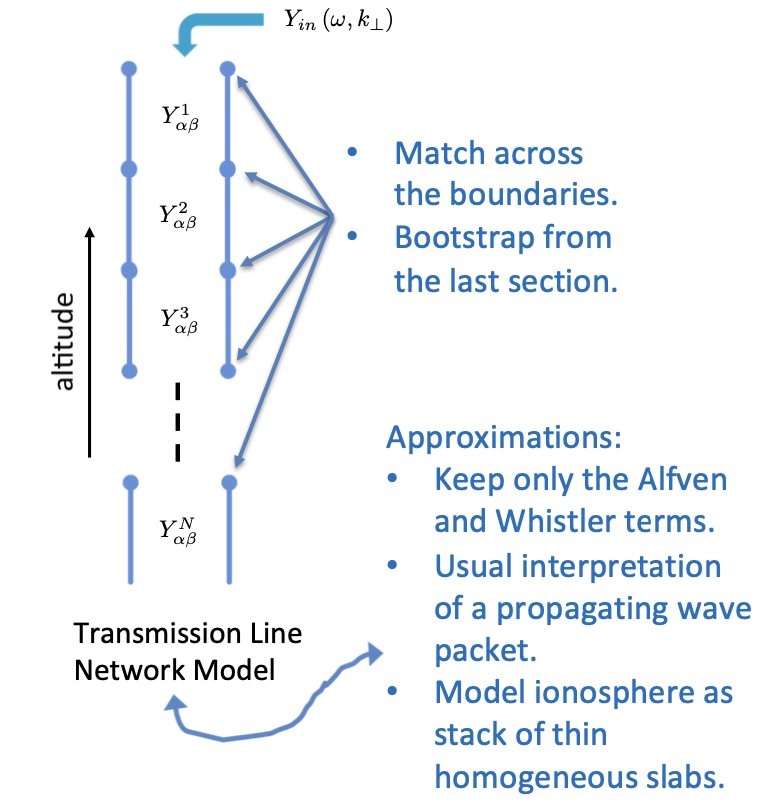
Of these two, the Whistler wave only propagates in the E region. So a signal arriving from the magnetosphere must arrive in the form of an Alfvén wave, and the magnetosphere-ionosphere coupling problem for our gedankenexperiment (Episode I) takes on the form shown in Figure 2. An ideal (non-collisional) Alfvén wave is incident from the magnetosphere, and in order to satisfy all the usual boundary conditions, the transmitted signal will generally be composed of both the (collisional) Alfvén and Whistler waves.

Figure 4: Panels a and b: Calculation of phase rotation and dissipation through the vertically-inhomogeneous ionosphere. Panel c: Total phase rotation versus transverse wavelength, for two different electron density profiles, and the same collision-frequency profiles as Figure 3.

Now we are in a position to test the electrostatic criteria (1). Figure 3 shows the wave-Pedersen conductivity (iY0kz) for both modes along with the usual (zero-frequency) Pedersen conductivity (σP), plotted versus altitude for a typical ionospheric-profile of collision-frequencies (profiles given in Cosgrove (2016), and for this example we take λ = 100 km and ne = 1011 m-3). Neither mode agrees very well at all, and so the third electrostatic criteria is not satisfied for either wave-mode.

To examine the first electrostatic criteria (λ≫ l) we calculate the minimum possible phase-rotation for a
signal traversing the ionosphere. That is, using the numerical results obtained from setting ωjr (k⃗, 2π/λjz) = ω0, we integrate the inverse of λjz over altitude, from 400 km down to 100 km, while choosing the longest wavelength mode at each altitude. This “best case” calculation is illustrated in Panel a of Figure 4, where the vertical dashed-black line indicates the altitude for switching from the Alfvén to the Whistler wave.

This phase rotation is analogous to the argument for the tangent function that appears in the electrostatic criteria (1), except that the ionosphere is now vertically inhomogeneous. The results are summarized in panel c of Figure 4, by plotting the best-case phase rotation versus transverse wavelength for two different electron density (ne) profiles. It is found that the phase rotation can exceed 90°, even for transverse wavelengths as long as 100 km. Since tan 90° = ∞, this represents a complete failure for the first of the electrostatic criteria.

With respect to the second electrostatic criteria (ldz ≫ l), a similar analysis (Panel b of Figure 4) finds that this criteria is nearly satisfied, that is, it is satisfied by the Whistler wave, and with the exception of the lower E region at longer wavelengths, it is also satisfied by the Alfvén wave. This result gives rise to the idea that the Whistler wave dominates in the lower E region, and the Alfvén wave in the region above, such that there may be an important transitional effect.

Thus we have answered the first three questions posed in the last paragraph of Episode I, and in all three cases the answers speak against electrostatic theory in a very strong way. However, we might continue to wonder whether a more general form of electrostatic theory, such as electrostatic wave theory, might be sufficient to salvage the situation. This question turns out to be tied up with the question of the actual, vertical-inhomogeneity of the ionosphere, and of the interaction between the two modes that it causes. We will address both these questions in Episode III, and in the process we will recover the most rigorous model ever for the ionospheric conductance, which must needs be an electromagnetic model.


by Russell Bonner Cosgrove


References

Cosgrove, R. B. (2016), Does a localized plasma disturbance in the ionosphere evolve to electrostatic equilibrium? Evidence to the contrary, J. Geophys. Res., 121, doi: https://doi.org/10.1002/2015JA021672.

Cosgrove, R. B. (2022), An electromagnetic calculation of ionospheric conductance that seems to override the field line integrated conductivity, Zenodo and ArXiv, doi: 10.48550/ARXIV.2211.10818, 10.5281/Zenodo.7416494.